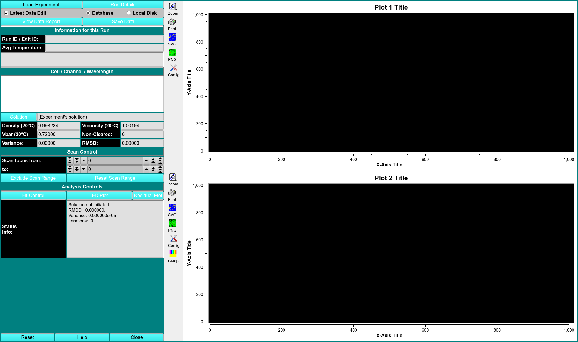
2-D Spectrum Analysis
This module enables you to perfrom 2DSA on a chosen experimental data set. Upon completion of an analysis fit, there are several plots avaliable: experiment, simulation, overlayed experiment and simulation, residuals, time-invarient noise, radially-invariant noise, and 3-D model.
The 2DSA method is used for composition analysis of sedimentation velocity experiments. It can generate sedimentation coefficent, diffusion coefficient, frictional coefficient, f/f0 ratio, and molecular weight distributions. The distributions can be plotted as 3-D plots, with the third dimension representing the concentration of the solute found in the composition analysis. The set of all such final calculated solutes for a model which are used to generate a simulation via Lamm equations. This simulation is then plotted overlaying a plot of the experimental data.
Each 2DSA pass can be repeated for a specificed number of refinement iterations These iterations, in turn, can be repeated for a specified number of meniscus points or Monte Carlo iterations.
Each refinement iteration proceeds over a defined grid of \(s\) and \(f/f0\) values. That grid is divided into subgrids as defined by a number of grid refinements in each direction.
CONTROLS
\(\textbf{Fit Control}\)
2DSA Fit Control
The parameters of this dialog define and control an analysis run to find the set of solutes that best fits experimental data.
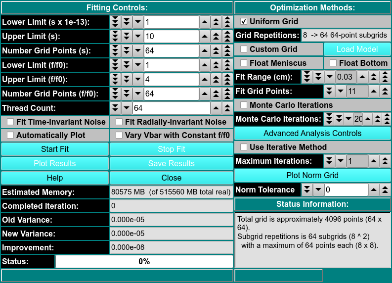
FITTING CONTROLS
\(\textbf{Lower/Upper Limit (s)}\) Set a lower/upper lmit of sedimentation coefficient values to scan.
\(\textbf{Number Grid Points (s)}\) Set the total grid count of sedimentation coefficient points.
\(\textbf{Lower/Upper Limit (f/f0)}\) Set a lower/upper lmit of frictional ratio values to scan.
\(\textbf{Number Grid Points (f/f0)}\) Set the total grid count of frictional ratio points.
\(\textbf{Thread Count}\) Specify by counter the number of threads to use for computations. This value is the total number of worker threads used at one time.
\(\textbf{Fit Time-Invarient Noise}\) Check this box if you want to calculate time-invarient noise.
\(\textbf{Fit Radially-Invarient Noise}\) Check this box if you want to calculate radially-invarient noise.
\(\textbf{Automatically Plot}\) Check this box if you want plot dialogs to automatically open at the completion of all calculations.
\(\textbf{Vary Vbar with Constant f/f0}\) Check this box if you want to vary vbar while holding f/f0 constant.
OPTIMIZATION METHODS
\(\textbf{Uniform Grid}\) Check this box if Uniform Grid is your preferred optimization method.
\(\textbf{Custom Grid}\) Check this box if you wish to have a custom grid as your preferred optimization method.
\(\textbf{Float Meniscus/Bottom}\) Check this box if you wish to wrap the refinement iterations in outer interactions of meniscus/bottom scans. Checking this option means that Monte Carlo may not be chosen.
\(\textbf{Load Model}\)
\(\textbf{Fit Range}\)
\(\textbf{Fit Grid Points}\)
\(\textbf{Monte Carlo Iterations}\) Select a number of Monte Carlo interations to perform. A seperate model is produced from each iteration.
\(\textbf{Advanced Analysis Controls}\)
\(\textbf{Use Iterative Method}\) Check this box if you want to refine anlysis fits with multiple refinement iteractions.
\(\textbf{Maximum Iterations}\) Select the number of maximum number of refinement iterations. This number may not be reached if subsequent iterations achieve the same set of computed solutes or if their variances differ by a very small amount.
\(\textbf{Plot Norm Grid}\)
\(\textbf{Norm Tolerance}\)
STATUS INFORMATION
\(\textbf{Estimated Memory}\) Text showing a memory use estimate based on chosen parameters.
\(\textbf{Completed Iteration}\) Display of the last completed refinement iteration completed.
\(\textbf{Old Variance}\) The variance value of the previous iteration.
\(\textbf{New Variance}\) The variance value of the last completed iteration.
\(\textbf{Improvement}\) The difference between the variance value from the last iteration and the one preceeding it.
\(\textbf{3-D Plot}\) Open a control window for a 3-D dimensional plot of the final computed model.
\(\textbf{Residual Plot}\) Open a plot dialog for a far more detailed set of results plots.
\(\textbf{Status Info}\) This text window displays continually updated summaries of computational activity and results.