Our modeled solution will be affected by random noise, time-invarient noise, the avaliable signal, and its ratio to the random noise. How then can we deal with the uncertainty of our solutions resolution?

First, we can improve the signal to noise ratio. This can be done by:

1. Obtaining lots of high quality data

2. Exploiting the entire dynamic range of the aquisition system

3. Reducing noise and only useing a well functioning instrument

4. removing systematic noise from experimental data

Additionally, we can:

• Replace fitting parameters with experimentally determinded values from seperate experiments

• Explore the parameter space with a grid method, than parsimoniously regulaize solution with GA, and use Monte Carlo to explore confidence regions

• Perform global fits for multiple experimental conditions to improve singal

There are three ways to reduce or eliminate noise to reduce the number of solutions.

1. Fit the noise.

2. Maintain an exceptionally well tuned instrument.

3. Design your experiment to optimize the quality of data.

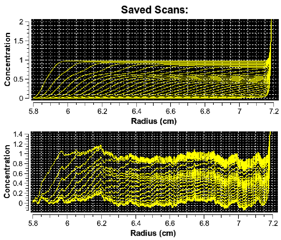
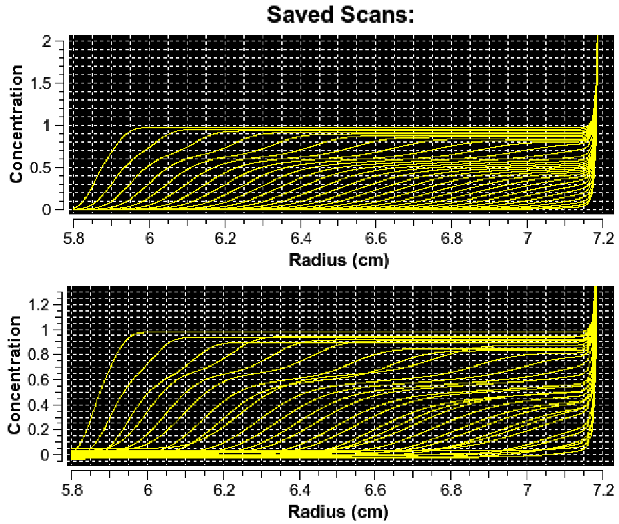
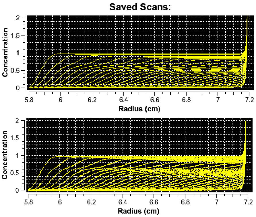
Types of Noise

There are at least three types of noise to consider when perfomring SV-AUC experiments:¹

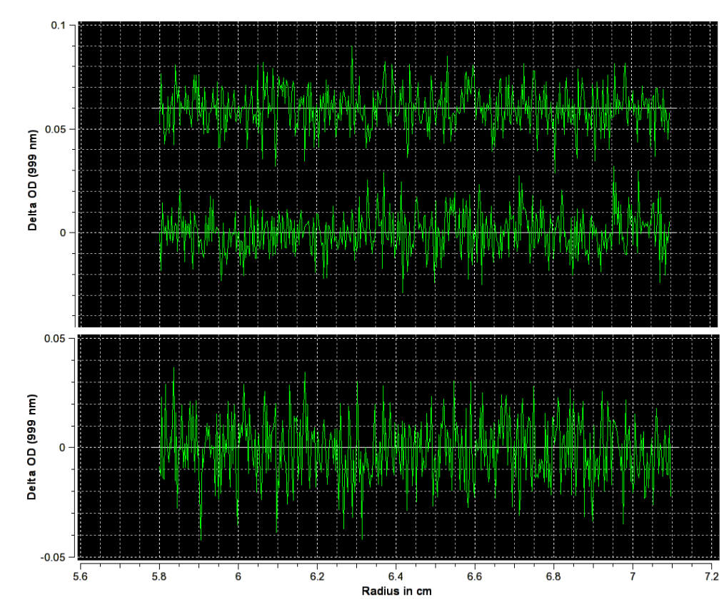
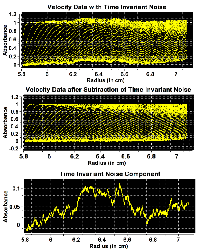
1. \(\textbf{Time-invariant noise}\) which produces a constant offset at a fixed radial position, and is identically valued at every observation. This type of noise is caused by imperfections in the optical track; for example, a fingerprint or scratch on a sample cell window.

   Lorem ipsum dolor sit amet, consectetur adipiscing elit, sed do eiusmod tempor incididunt ut labore et dolore magna aliqua. Ut enim ad minim veniam, quis nostrud exercitation ullamco laboris nisi ut aliquip ex ea commodo consequat. Duis aute irure dolor in reprehenderit in voluptate velit esse cillum dolore eu fugiat nulla pariatur. Excepteur sint occaecat cupidatat non proident, sunt in culpa qui officia deserunt mollit anim id est laborum.

1. \(\textbf{Radially-invaraient noise}\) which has a constant offset at a fixed time, and has identical calues at every radial position.

   Lorem ipsum dolor sit amet, consectetur adipiscing elit, sed do eiusmod tempor incididunt ut labore et dolore magna aliqua. Ut enim ad minim veniam, quis nostrud exercitation ullamco laboris nisi ut aliquip ex ea commodo consequat. Duis aute irure dolor in reprehenderit in voluptate velit esse cillum dolore eu fugiat nulla pariatur. Excepteur sint occaecat cupidatat non proident, sunt in culpa qui officia deserunt mollit anim id est laborum.

2. \(\textbf{Normally distribued noise}\) from non-linearity in the optics, intensity fluctuations of the lamp flashes, refractive artifacts, and systematic contributions of unknown sources.

   Lorem ipsum dolor sit amet, consectetur adipiscing elit, sed do eiusmod tempor incididunt ut labore et dolore magna aliqua. Ut enim ad minim veniam, quis nostrud exercitation ullamco laboris nisi ut aliquip ex ea commodo consequat. Duis aute irure dolor in reprehenderit in voluptate velit esse cillum dolore eu fugiat nulla pariatur. Excepteur sint occaecat cupidatat non proident, sunt in culpa qui officia deserunt mollit anim id est laborum.

Fitting Noise

Lorem Ipsum

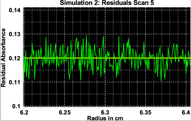
SedFit uses an algebraic noise decomposition strategy based on direct least-squares modelling. There is no increase in the statistical noise, and you can obtain explicit estimates for the magnitude of the systematic noise components. However, there are two limitations to keep in mind when using this method of systematic noise decomposition:

1. Calculated systematic noise is an estimate and model dependent.

we can only assume the calculated noise to reflect a true baseline signal if we have a good fit for our sedimentation data.

1. There is no fundamental difference in the effect of systematic noise on the data analysis from a time-difference analysis.

Fortunately, for larger data sets, the baseline is usually well-determined, and so the issues described above are not largely problematic.

TI Noise in TI Signals

Work on this matter is being done by Saeed Mortezazadeh, post-doctoral fellow at the University of Lethbridge.

When performing equilibirum experiments, it is not possible to distinguish the time-invarient noise patterns from the signals due to the balancing of the sediment flux with the diffusion flux (Fick's Laws).

Solution 1: run empty cells and collect the intensity data patterns of each radial point and wavelength. The volume of the data collected must be significant (due to the presence of statistical noise in each scan) so that a time-invariant pattern can be averaged over all scans.

It is important to note that while the AUC Optima claims to emit light with a one nanometer resolution over a 190 nm to 700 nm range, different patterns can be observed in both the shape and intensity of scans. This is especially prevelant at lower wavelengths and it seems that the monochromatic optical system does not completely split the light, and as a result, the light emitted at a particular wavlength can be paritally mixed with neighbouring wavelengths.

The intensity of each scan is calculated by averaging the intensity of all radial points:

The root mean square deviation (RMSD) is calculated to qantify the shape of each scan:

The mean and RMSD overlapp of scans are clearly visible between neighbouring wavelengths.

How do we detemine which scan belongs to which wavelength?

1. Calculate the histogram (probability distribution function) of the RMSD values for each wavelength using the core density equilibirium method.

2. Scans with similar scans are consider to be in a cluster; histograms are used to cluster scans of all wavelengths.

3. The main scans of corresponding scans are assumed to be the scans belonging to the cluster with the highest probability distribution.

4. If the non-original clusters overlap with the main cluster of adjacent wavelengths, the corresponding scans are transferred to the adjacent wavelength.

The procedure for this method is imbedded in UltraScan, and the steps are outlined here.